Data Models, Querys, and Storage - Part 1 of Designing Data-Intensive Applications

Anthoer book summary/review!

Layout of the Whole Book

The book is arranged into these parts:

1. Fundamental ideas that underpin the design of data-intensive applications.
   • What we’re actually trying to achieve: reliability, scalability, and maintainability; how we need to think about them; and how we can achieve them.
   • Comparisons of different data models and query languages
   • Storage engines how databases arrange data on disk so that we can find it again efficiently.
   • Encoding and evolution of schemas over time.
2. Distributed Data
   • Replication, partitioning/sharding
   • Transactions
   • Consistency and consensus
   • Batching
   • Streaming

This blog post only talks about part 1.

Data Models and Query Languages

The book talks about various query languages other than SQL which can be referred from the book so we are not going to talk about them here. Essentially there are a few general-purpose data models for data storage and querying including relational model (SQL), the document model like JSON and XML (NoSQL), and graph-based model. The idea is that relational model is good at modeling relations (called tables in SQL), where each relation is an unordered collection of tuples (rows in SQL); the document model is good at modeling documents or “objects” in programming; when it comes to many-to-one and many-to-many relationships, graph-based model does the best job.

Storage and Retrieval

SSTables and LSM-Trees

SSTable stands for Sorted String Table. The idea is that we keep an in-memory table where every key is mapped to a byte offset in the data file. Whenever you append a new key-value pair to the file, you also update the table to reflect the offset of the data you just wrote (this works both for inserting new keys and for updating existing keys). When you want to look up a value, use the table to find the offset in the data file, seek to that location, and read the value. It’s basically an append-only log. The key idea is that the sequence of key-value pairs is sorted by key.

How do you get your data to be sorted by key in the first place? Use a balanced BST!

We can now make our storage engine work as follows:

• When a write comes in, add it to an in-memory balanced tree data structure (for example, a red-black tree). This in-memory tree is sometimes called a memtable.
• When the memtable gets bigger than some threshold—typically a few megabytes—write it out to disk as an SSTable file. This can be done efficiently because the tree already maintains the key-value pairs sorted by key. The new SSTable file becomes the most recent segment of the database. While the SSTable is being written out to disk, writes can continue to a new memtable instance.
• In order to serve a read request, first try to find the key in the memtable, then in the most recent on-disk segment, then in the next-older segment, etc.
• From time to time, run a merging and compaction process in the background to combine segment files and to discard overwritten or deleted values.

How do we avoid eventually running out of disk space? A good solution is to break the log into segments of a certain size by closing a segment file when it reaches a certain size, and making subsequent writes to a new segment file. We can then perform compaction on these segments. Compaction means throwing away duplicate keys in the log, and keeping only the most recent update for each key. Moreover, since compaction often makes segments much smaller (assuming that a key is overwritten several times on average within one segment), we can also merge several segments together at the same time as performing the compaction. Segments are never modified after they have been written, so the merged segment is written to a new file. The merging and compaction of frozen segments can be done in a background thread, and while it is going on, we can still continue to serve read and write requests as normal, using the old segment files. After the merging process is complete, we switch read requests to using the new merged segment instead of the old segments—and then the old segment files can simply be deleted.

If you want to delete a key and its associated value, you have to append a special deletion record to the data file (sometimes called a tombstone). When log segments are merged, the tombstone tells the merging process to discard any previous values for the deleted key.

if the database crashes, the most recent writes (which are in the memtable but not yet written out to disk) are lost. In order to avoid that problem, we can keep a separate log on disk to which every write is immediately appended. That log is not in sorted order, but that doesn’t matter, because its only purpose is to restore the memtable after a crash. Every time the memtable is written out to an SSTable, the corresponding log can be discarded.

Append-only log with SSTable has several advantages:

• Appending and segment merging are sequential write operations, which are generally much faster than random writes, especially on magnetic spinning-disk hard drives. To some extent sequential writes are also preferable on flash-based solid state drives (SSDs)
• Concurrency and crash recovery are much simpler if segment files are append-only or immutable. For example, you don’t have to worry about the case where a crash happened while a value was being overwritten, leaving you with a file containing part of the old and part of the new value spliced together.
• Merging segments is simple and efficient, even if the files are bigger than the available memory. The approach is like the one used in the mergesort algorithm. You start reading the input files side by side, look at the first key in each file, copy the lowest key (according to the sort order) to the output file, and repeat. This produces a new merged segment file, also sorted by key. What if the same key appears in several input segments? Remember that each segment contains all the values written to the database during some period of time. This means that all the values in one input segment must be more recent than all the values in the other segment (assuming that we always merge adjacent segments). When multiple segments contain the same key, we can keep the value from the most recent segment and discard the values in older segments.
• Merging old segments avoids the problem of data files getting fragmented over time.
• Lookup is fast as it’s basically a binary search

B-Trees

Like SSTables, B-trees keep key-value pairs sorted by key, which allows efficient key-value lookups and range queries. But that’s where the similarity ends: B-trees have a very different design philosophy. The log-structured indexes we saw earlier break the database down into variable-size segments, typically several megabytes or more in size, and always write a segment sequentially. By contrast, B-trees break the database down into fixed-size blocks or pages, traditionally 4 KB in size (sometimes bigger), and read or write one page at a time. This design corresponds more closely to the underlying hardware, as disks are also arranged in fixed-size blocks. Most databases can fit into a B-tree that is three or four levels deep, so you don’t need to follow many page references to find the page you are looking for. (A four-level tree of 4 KB pages with a branching factor of 500 can store up to 256 TB.)

The basic underlying write operation of a B-tree is to overwrite a page on disk with new data. It is assumed that the overwrite does not change the location of the page; i.e., all references to that page remain intact when the page is overwritten. This is in stark contrast to log-structured indexes such as LSM-trees, which only append to files (and eventually delete obsolete files) but never modify files in place.

In order to make the database resilient to crashes, it is common for B-tree implementations to include an additional data structure on disk: a write-ahead log (WAL, also known as a redo log). This is an append-only file to which every B-tree modification must be written before it can be applied to the pages of the tree itself. When the data‐ base comes back up after a crash, this log is used to restore the B-tree back to a consistent state

Comparing B-Trees and LSM-Trees

As a rule of thumb, LSM-trees are typically faster for writes, whereas B-trees are thought to be faster for reads. Reads are typically slower on LSM-trees because they have to check several different data structures and SSTables at different stages of compaction.

OLTP and OLAP

OLTP stands for online transaction processing and OLAP stands for online analytic processing. We can compare characteristics of the two as following

Property	OLTP	OLAP
Main read pattern	small number of records per query, fetched by key	Aggregate over large number of records
Main write pattern	Random-access, low-latency writes from user input	Bulk import (ETL) or event stream
Primarily used by	End user/customer, via web application	Internal analyst, for decision support
What data represents	Latest state of data (current point in time)	History of events that happened over time
Dataset size	Gigabytes to terabytes	Terabytes to petabytes

Data Warehousing and Column-Oriented-Storage

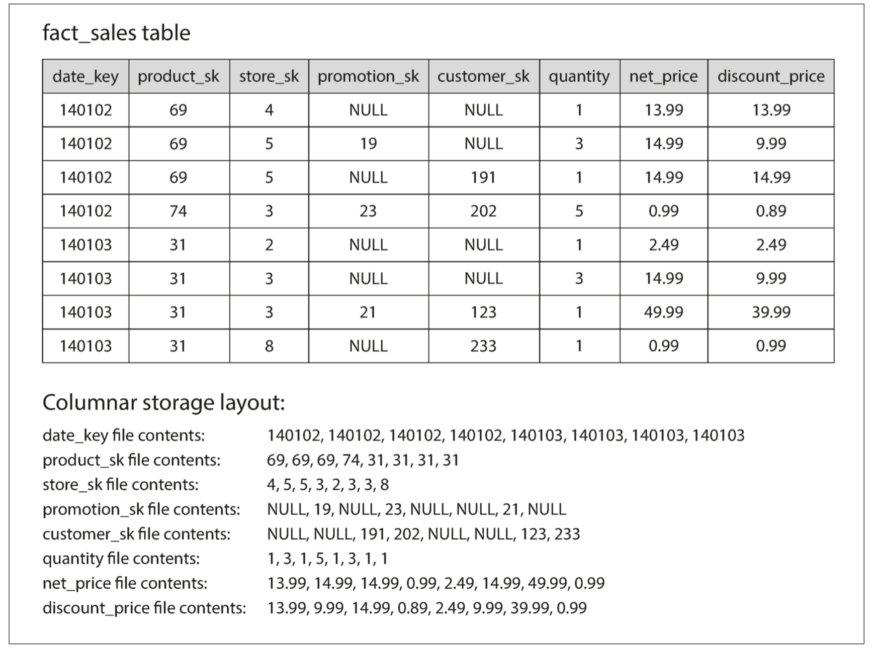
The example schema following shows a data warehouse that might be found at a grocery retailer. At the center of the schema is a so-called fact table (in this example, it is called fact_sales). Each row of the fact table represents an event that occurred at a particular time (here, each row represents a customer’s purchase of a product). If we were analyzing website traffic rather than retail sales, each row might represent a page view or a click by a user.

In a typical data warehouse, tables are often very wide: fact tables often have over 100 columns, sometimes several hundred. Dimension tables can also be very wide, as they include all the metadata that may be relevant for analysis—for example, the dim_store table may include details of which services are offered at each store, whether it has an in-store bakery, the square footage, the date when the store was first opened, when it was last remodeled, how far it is from the nearest highway, etc. Although fact tables are often over 100 columns wide, a typical data warehouse query only accesses 4 or 5 of them at one time (“SELECT *” queries are rarely needed for analytics). But in most OLTP databases, storage is laid out in a row-oriented fashion: all the values from one row of a table are stored next to each other. Document databases are similar: an entire document is typically stored as one contiguous sequence of bytes. So we need another layout of our storage engine, which is column-oriented storage.

The idea behind column-oriented storage is simple: don’t store all the values from one row together, but store all the values from each column together instead. If each column is stored in a separate file, a query only needs to read and parse those columns that are used in that query, which can save a lot of work. This principle is illustrated below.

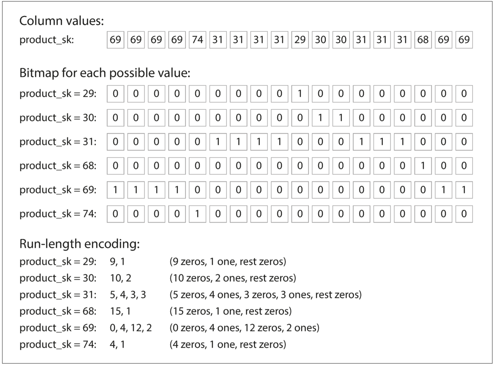
Besides only loading those columns from disk that are required for a query, we can further reduce the demands on disk throughput by compressing data. Fortunately, column-oriented storage often lends itself very well to compression: columns often look quite repetitive (for example, a retailer may have billions of sales transactions, but only 100,000 distinct products), so we can use a bitmap to encode them.

If n is very small (for example, a country column may have approximately 200 distinct values), those bitmaps can be stored with one bit per row. But if n is bigger, there will be a lot of zeros in most of the bitmaps (we say that they are sparse). In that case, the bitmaps can additionally be run-length encoded, as shown below.

Note: Cassandra and HBase have a concept of column families, which they inherited from Bigtable. However, it is very misleading to call them column-oriented: within each column family, they store all columns from a row together, along with a row key, and they do not use column compression. Thus, the Bigtable model is still mostly row-oriented.

Summary

On a high level, we saw that storage engines fall into two broad categories: those optimized for transaction processing (OLTP), and those optimized for analytics (OLAP). There are big differences between the access patterns in those use cases:

• OLTP systems are typically user-facing, which means that they may see a huge volume of requests. In order to handle the load, applications usually only touch a small number of records in each query. The application requests records using some kind of key, and the storage engine uses an index to find the data for the requested key. Disk seek time is often the bottleneck here.
• Data warehouses and similar analytic systems are less well known, because they are primarily used by business analysts, not by end users. They handle a much lower volume of queries than OLTP systems, but each query is typically very demanding, requiring many millions of records to be scanned in a short time. Disk bandwidth (not seek time) is often the bottleneck here, and column- oriented storage is an increasingly popular solution for this kind of workload.

On the OLTP side, we saw storage engines from two main schools of thought:

• The log-structured school, which only permits appending to files and deleting obsolete files, but never updates a file that has been written. Bitcask, SSTables, LSM-trees, LevelDB, Cassandra, HBase, Lucene, and others belong to this group.
• The update-in-place school, which treats the disk as a set of fixed-size pages that can be overwritten. B-trees are the biggest example of this philosophy, being used in all major relational databases and also many nonrelational ones.

We then took a detour from the internals of storage engines to look at the high-level architecture of a typical data warehouse. This background illustrated why analytic workloads are so different from OLTP: when your queries require sequentially scanning across a large number of rows, indexes are much less relevant. Instead it becomes important to encode data very compactly, to minimize the amount of data that the query needs to read from disk. We discussed how column-oriented storage helps achieve this goal.